Finite Difference Groundwater Modeling in Python
Previously Matlab-based graduate course at TUDelft
Prof. dr.ir. T.N.Olsthoorn
Dec 31, 2016, 24 May 2016
Abstract ABSTRACT
This syllabus explains the theory behind numerical groundwater modeling and how to make your own finite difference groundwater models in Python. The theory is equally well applicable to other computations and computer language environments like Octave, Scilab and Python. This syllabus aims at providing in-depth insight in numerical modeling of groundwater. It is also base for exercises in the master course CT5440, Geohydrology 2, of the TU-Delft. Although the structure is kept general, and, therefore applicable also to other times of models like finite element models and even surface water flow models, its focus is on finite difference models.
During the course, the student will build his or her own finite difference model in Python. The student will see how flat, axially symmetric, 3D, steady-state and transient models are related. He will also learn how initial and boundary conditions are introduced. Special attention is given to effective treatment of fixed-head boundaries. The models are small Python functions, elegant yet powerful, i.e. capable of simulating simple and small as well as complex and and large groundwater flow problems.The examples serve to demonstrate some things what may be done as well to verify their accuracy including some pitfalls and how to avoid them.
A real world modeling project is generally preceded by a stage where insight is gained into the answers to be provided and the structure and processes relevant in the system to be modeled. In a subsequent step, one or more conceptual models will be made to simulate groundwater behavior under a number of stresses of various types in terms of heads and flows that force the groundwater in the system. Such stresses are surface water elevations, recharge, evaporation, pumping and drainage. The questions to be answered in combination with the relevant complexity of the system also determine the detail of the model mesh to be used, both in space and time. Much time is generally spent on acquiring input and putting it into the form in which the model can use it. Nowadays, much information is often directly drawn from databases and already filled GIS systems, including remotely sensed data such a rain radar. However, one must remain very critical regarding the relevance and correctness of each data item with respect to the modeling problem at hand. In the end, the modeler is responsible for the outcomes, not the model or the computer. The results and predictions often stand at the basis of decisions that will affect livelihoods of people as well as habitats of plants and animals. Lack of time prohibits dealing with with such extended real-world problems in this course. Insight into the internal behavior of the model and the ability to verify its outcomes are more relevant to the engineer, and therefore, is the focus of this syllabus.
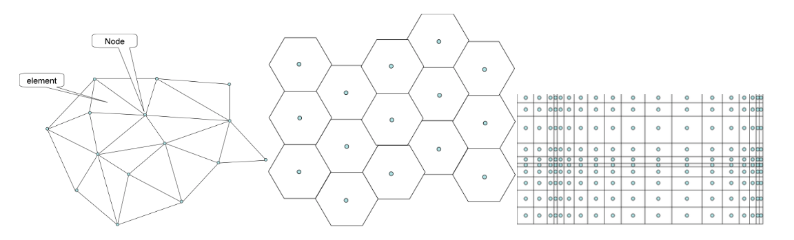
mesh1
Figure: Different model meshes (grid). Left: a finite element triangular network with the nodes at the element corners. Middle: a hexagonal finite difference network with nodes in the center of hexagonal cells. Right: a rectangular finite difference network with nodes in the center of the cells. Area properties are generally specified for elements in the finite element method and for cells in the finite difference method. Heads and flows are generally specified at the nodes of the finite element method and at the cell centers of the finite difference method.
Because MODFLOW, the open-source groundwater model of the United States Geological Survey, is worldwide the most used groundwater model, we’ll stay close to its approaches and terminology so that the MODFLOW manual will look familiar to the student. MODFLOW is a fully-implicit 3D finite difference model written in FORTRAN. It can be downloaded together with its manual and source code from HTTP://water.USGS.gov/ogw/modflow.
The Python environment is far more expressive and, from that point of view more powerful than FORTRAN meaning we can set-up a powerful MODFLOW-like model in Python within a few tens of lines of code in way we can fully understand; MODFLOW requires thousands of lines of FORTRAN that are difficult to grasp unless you are a software engineer with expertise in FORTRAN and modeling at the same time. Python has the power to build a model line by line, interactively, while testing each part of the code immediately on screen, supported by its very powerful debugger, which points at the location where a problem occurred and allows full inspection of the circumstances that caused it.
Next to modeling, Python is also a powerful environment to visualize modeling results. Therefore, outside Python no additional packages are required. Some Python knowledge has, of course, to be acquired during the course. There exist very good Python books, documentation and tutorials on the web; vertually any question related to Python can be “googled” to find useful ansers..
Numerical groundwater modeling
We will start with a general description of groundwater modeling and then derive an actual numerical model, which will finely be converted into a finite difference model by choosing the network and the way the so-called conductance between model cells are computed. The general overview that follows is valid for all kinds of numerical models. We will follow the general approach as long as possible because it provides the best insight with the least clutter.
Numerical models divide the space to be modeled into an often large number subspaces, called elements in the Finite Element Method (FDM) or cells in the Finite Difference Method (FDM). The properties of each element or cell are specified and generally taken constant within. In the FEM, the heads will be computed at the nodes, whereas in the FDM they will be computed at the cell centers. In the FEM, flows will be computed between the nodes, whereas in the FDM they will be computed at the cell faces between adjacent elements. In the FDM the governing partial differential equation directly discretized on the grid, which takes the form of a water balance equation of each cell and, hence, for the model as a whole. The FEM requires that the partial differential equation integrated over each element is satisfied. Solving the model means adjusting all non-fixed nodal or cell heads such that the water balance over all cells and elements are satisfied simultaneously. The FEM and FDM generally lead to different grid shapes, see [fig:Different-model-meshes]. The elements associated with the FEM may be of arbitrary shape, while the shape in the FDM is generally more limited to regular hexagons or rectangular for instance. However, the newest version of MODFLOW, MODFLOW-USG which stands for “Un Structured Grid”, brings finite elements and finite differences much closer together by allowing arbitrarily shaped grids, but this is considered beyond the scope of this syllabus.
To stay close to MODFLOW, we will make a finite difference model with rectangular or block-shaped cells in which the properties of the subsurface are assumed constant and at the center of which the heads are computed. The flows are computed at the cell faces, i.e. between adjacent cells.
Although it is straightforward to derive a full 3D finite difference model from the onset, we start with a 2D model for simplicity, where we divide the subsurface into Ny rows and Nx columns. The cell sizes thus defined may vary from column to column and from row to row. The thickness in the z-direction may vary if desired.. This configuration is shown in right-hand picture of figure [fig:Different-model-meshes]. This approach is easy to understand and easy to implement.
The finial result of any of the possible derivations of the model equations, no matter if they are for a finite element model or a finite difference model, comes down to a system of equations, each of which is the water balance for a node or cell of that model. This system of equations represents all nodal water balances. Solving the model is fulfilling these water balances for all models simultaneously. This is achieved computing the unknown heads in the nodes/cells that make all nodal/cell water balances match simultaneously.
The FDM is derived by directly writing down equations for the water balance for the nodes; the FEM takes a more general approach by requiring the governing partial differential equation, which is the water balance on infinitesimal scale, to be optimally fulfilled within all of the elements. The the FEM is more complicated in deriving its equations and setting up the model, but the bonus is more flexibility in element shapes.
In the end, any numerical groundwater model yields a set of water balances, one for each node. This is true for the FEM, the FDM as it is for any surface water model. In all such models the the space between nodes is replaced by links model types differ only in the way how this is done. In any case, the number of equations, as well as the number of unknowns, equals the number of non-fixed nodes, equals the number of water balances. A finite difference model of 300 rows, 300 columns and 10 layers thus has 0.9 million equations and the same order of unknowns.
Figure [fig:Model-node] shows some of the nodes (or cell centers) of an arbitrary finite element or finite difference model. For one node or cell, with index number i, the adjacent nodes are shown to which it is directly connected, that is, they share one element edge in the FEM or one cell face in the FDM (or one canal or river section in a surface water model). The only difference between these types of models is the way in which the connections are computed. So most of the discussion about modeling and model construction can be done without bothering about these specific details, which is the line followed in this syllabus, because it is most general. For the sake of simplicity whenever the word node is used it can be read as a node in the FEM or equally as a cell center in the FDM.
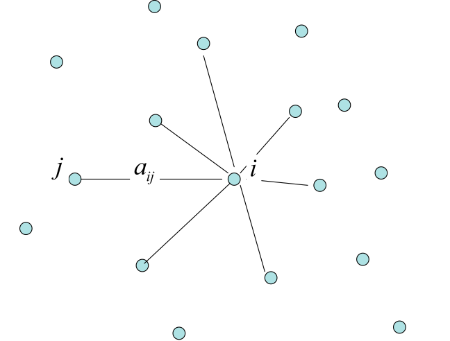 Figure: A model node with its surrounding connected
neighbors
Figure: A model node with its surrounding connected
neighbors
Just as general is, that the flow \(Q_{ij}\) from node i in the direction of adjacent node j with heads \(\phi_{i}\) and \(\phi_{j}\) respectively, is described by
\(C_{ij}\) [(L3/T)/L]} or [L2/T] is called the “conductance” and its reciprocal is the “resistance” \(\mbox{[L/(\ensuremath{L^{3}}/T)]}\). The conductance comprises the properties of the area between the connected nodes and their distance. In case the conductance is not constant, as is the case in a surface water model or in a groundwater model with a water table in which the transmissivity is not known a priori, this flow must be computed iteratively.
The physical meaning of the conductance is obvious: it is the flow of water \([L3/T]\) from node \(i\) to node \(j\) in case the head difference \(\phi_{i}-\phi_{j}\) [L] equals 1 [L]. The actual dimension depends on the system used, i.g meters and days or feet and hours.
The steady state water balance of an arbitrary node i in the numerical model is described by the following equation
Where \(Q_{i}\) is the inflow to the node or cell from the outside world and the left hand side is the combined outflow from the node or cell to all its neighbors. Hence inflow from the outside world into the model is taken positive. The left -hand side thus represents the flow from node i through the model towards its connected neighbors. We will deal with transient models later.
The nodal inflow \(Q_{i}\), is the sum of all inflows of water from the outside world into node \(i\) minus the extractions of water from node \(i\) to the the outside world. Therefore, \(Q_{i}\) combines recharge, injections, extractions, leakage, drainage and so on, summed over and integrated over the space attributed to the node (FEM) or cell (FDM).
Using conductances, the nodal water balance becomes:
Notice that \(i\) and \(j\) run over all the nodes of the model. This equations expresses that node \(i\) may be connected to any or all other nodes of the model no matter how far apart. Of course, in an ordinary model each node is only connected to its direct neighbors. Therefore, most of the conductances \(C_{ij}\) are zero. In case a node has n connected neighbors, only \(n+1\) of these conductances are non-zero for each node. Therefore, of a model with \(N\) nodes has \(N\times N\) possible connections of which \(N\) with node \(i\). These connections, and hence, conductances, potentially fill a matrix of \(N\) rows and \(N\) columns. Notice that a finite difference model with a grid consisting of \(N_{x}\) rows by \(N_{y}\) columns and \(N_{z}\) layers, ha \(N=N_{x}\times N_{y}\times N_{z}\) cells, and, therefore, this \(N\times N\) array can easily exceed the memory capacity of any available computer. For instance, a model having “only” 300 rows, 300 columns and 10 layers has \(N=0.9\) million cells and hence the \(N\times N\) array of possible conductances has \(N^{2}=0.81\times10^{12}\) entries. With, with 4 bytes per value to be stored this would require a computer memory of \(3\times10^{12}\) bytes or about 3 terabyte. This is huge for any internal computer memory. However, if we only store the non-zero values, then the maximum number of conductance to be stored it tremendously reduced. In a 3D finite difference model the maximum number of connected neighbors of any cell is 7. This implies that the number of non-zero values can be no more than \(7\times N\) , i.e. \(7\times4\times0.81\times10^{6}\approx\ 30\) Mb in the example model. This memory storage peanuts on even a modern PC with for instance 8 GB internal memory. In fact the array of conductances is extremely sparse. In this case the fraction of non-zero values is at most \(7\times N/N^{2}=7/N\approx10^{-5}\) or 0.001%.. We will therefore make use of this sparsety when storing the system matrix and solving the model, because, if we do not do this, our computer could not even handle a small size model!
Writing out the above balance equation yields
or
where
The physical meaning of diagonal matrix element \(C_{ij}\) is the amount of water flowing from node i to all its adjacent nodes if the head in node i is exactly 1 m higher than that of its neighbors.
Equation [eq:nodal-water-balance-with-conductances] can be written compactly as follows:
where the sum taken over all matrix elements in a row equals zero
which means that the flow from node \(i\) to node \(j\) with \(\phi_{i}-\phi_{j}=1\) equals the flow from node \(j\) to node \(i\) when \(\phi_{j}-\phi_{i}=1\). Under special circumstances, this may not be true, in which case the model is non-linear and needs to be solved iteratively.
Equation [eq:system-equation-as-sum] is equivalent to the matrix equation
With \(\mathbf{C}\) the square coefficient or system matrix, which holds the conductances \(-C_{ij},\,i\ne j\) and \(C_{ii}\) as defined in equation [eq:Cii]. In a 3D finite difference model, both \(i\) and \(j\) may take values from 1 to \(N_{x}\times N_{y}\times N_{z}\). Therefore, the size of \(\mathbf{C}\) in such a model is \(N_{x}\times N_{y}\times N_{z}\) rows by \(N_{x}\times N_{y}\times N_{z}\) columns, which potentially is huge. \(\Phi\) is the column vector of still unknown heads at the nodes or cell centers (its size is \(1\times N_{x}N_{y}N_{z}\)) and \(\mathbf{Q}\) the column vector net nodal or cell inflows from the outside world, which has the same size as \(\Phi\)..
To fill the system matrix, we have to compute the conductances between all connected nodes and put their value into the matrix at location specified by \(i\) and \(j\). That is, \(-C_{ij}\) goes to row \(i\) and column \(j\), \(i\ne j\). When done, the coefficients for the diagonal, \(C_{ii}\), are computed by taking the negative sum of the no-diagonal elements in line \(i\) of the matrix, which representing node \(i\).
Before deriving the expressions for the conductances, and hence, the how to compute the elements in the system matrix, we consider the model’s boundary conditions.
To prevent having to deal with the zeros in over 99% of the system
matrix, Python’s scipy.sparse module offers sparse matrices and
sparse matrix functions. These sparse matrices work exactly like
ordinary matrices but they store only the non-zero elements.
Scipy.sparse also offers sparse matrix functions that know how to
handle sparse matrices and how to deal only with the non-zeros elements.
It is the sparse matrices that make computing of large numerical models
feasible on a PC.
Boundary conditions connect the model to the outside world, by linking nodes to heads outside the model or by specifying inflows and extractions, which can be of any type including wells, drainage, recharge and evaporation. Model nodes can also be linked to an outside head through a conductance \(\hat{C}\) or a resistance \(R=1/\hat{C}\). Such lines turn out to be a mixture of a fixed head and a fix flow boundary.
Exchange between model nodes and the outside world through flows is quite trivial: all net inflows to (negative if outflows from) the outside world, whatever their type, are directly added to the the inflow at the right-hand size of equation [eq:Model-equation]; i.e. all given inflows minus outflows to node \(i\) are added to \(Q_{i}\) in vector \(\mathbf{Q}\).
The other types of boundary condition deal with heads, such that the flow between the outside world and the model node is driven by the head difference, and, therefore, is a priori unknown. We treat this in a general way, i.e. by writing out how fixed heads in the outside world connect to nodes of the model through a conductance \(\hat{C}\). Heads that are fixed directly at a node of the model, i.e. fixed heads, become a limiting case in which the conductance approaches \(\infty\) or the resistance approaches zero. These heads can and will be handled separately in a way that speeds up the model and stabilizes it.
Consider flow \(Q_{ex,\,i}\) into node \(i\) from from a water body in the external to the model. Let the head in that water body be fixed and equal to \(h_{i}\) while the head \(\phi_{i}\) in the model at node \(i\) is unknown. This flow through the conductance \(\hat{C}_{i}\) between node and outside world equals
This flow can be simply added to the right-hand side of the model equation to give
in which the diagonal \(C_{ii}\) was taken out of the matrix for clarity (notice the sum indices).
Equation [eq:Qex] represents a net inward flow , just like the given inflow \(Q_{i}\).
This way, each model node may be connected to the outside world having arbitrary fixed heads (lakes, rivers and so on).
The constant part , \(\hat{C}_{i}h_{i}\), works exactly like a fixed inflow. The variable part, \(C_{i}\phi_{i}\), may be put to the left-hand side of the equation to yield
This boils down to adding \(\hat{C}_{i}\) to the diagonal matrix entry, \(C_{ii}\rightarrow C_{ii}+\hat{C}_{i}\).
In matrix form for direct in use in Python, using the subscript \(\mathbf{ghb}\) to indicate general head boundary
Where \(diag\left(\mathbf{\hat{C}_{g}}\right)\) is an \(N\times N\) diagonal matrix with the elements \(\hat{C}_{i}\). This is indeed equivalent to adding \(\hat{C}_{i}\) to the diagonal elements \(C_{ii}\). Notice that \(\hat{C}_{i}\ne0\) only where general head boundaries exist, but they can be associated with any cell in the model.
The boundary conditions explained in this section are so-called general head boundaries. In Modflow jargon they are abbreviated to GHB. Truly fixed-head boundaries are dealt with further down.
Modflow has two other variants of these general head boundaries: called drains (abbreviated to DRN) and rivers (abbreviated to RIV). DRNs differ form GHBs in that they only discharge when the head in the model is above the user-specified drain elevation. RIVs differ from GHBs in that the head difference that drives the flow from the river to the connected model node is limited to the water depth of the river; if the head in the model node declines below the river bottom, the river bottom is used instead of the head as explained below.
Drains and rivers thus make the model non-linear as they imply a switch, i.e. cut off or curtail flow depending on the head in the model. Such non-linearities are dealt with using iterative matrix solvers, so that the flows can be updated during the solution process. We will ignore iterative solvers in Python even when the model is non-linear and use a standard (sparse) matrix solver repeatedly when needed, until convergence is achieved. This mostly works faster.
As said above, drains work as general head boundaries as long as the head is above the drain elevation. When the head declines to below the local drain elevation, the flow is set to zero. For the DRN cells we thus need to specify a drain elevation, i.e. a vector \(\mathbf{h}_{\mathbf{drn}}\) next to the drain conductances \(\hat{\mathbf{C}}_{\mathbf{drn}}\). Of course, \(\hat{C}_{\mathbf{drn,i}}\ne0\) only for cells that have drains connected.
The switch may be implemented as a using Boolean vector \(\mathbf{b}_{\mathbf{drn}}\) which contains true (or 1) for all cells where \(\Phi>\mathbf{h}_{\mathbf{drn}}\) and false (0) otherwise:
Hence, the drains are implemented as follows:
Notice that in Python, a Boolean true becomes 1 if used in arithmetic operations and false then becomes zero. The Boolean vector in the above equation should therefore be read as a vector of ones an zeros.
River boundaries are also general head boundaries as long as the head remains above the bottom of the river. When it falls below the river bottom, \(h_{B}\), the infiltration is assumed to pass through the unsaturated zone without suction from the fallen head. So, for an arbitrary river node:
writing \(b_{riv}=\phi>h_{bot}\) and \(\neg b_{riv}=\neg\left(\phi>h_{bot}\right)=\phi\le h_{bot}\)
or
In Python where \(\neg b_{riv}=1-b_{riv}\) this reduces to
Therefore MODFLOW-type rivers can be implemented as follows
Combining the three previous sections, the model equation with all general head, drain and river boundaries then becomes:
Equation [eq:system-equation-head-boundaries] specifies the complete model from which the heads may be solved directly in Python using the appropriate function (see actual Python code in subsequent chapters).
Combining for simplicity the contribution from the different head boundary conditions under :raw-latex:`\mathbf{\hat{C}}` and h, different, the solution of equation [eq:system-equation-head-boundaries] simplifies to:
where the backslash is “Matlab language” means: solve this set of equations for the unknowns at the left, but don’t necessarily invert the matrix left of the \ for computation efficiency reasons.
The column vector \(\mathbf{\hat{C}}\cdot\mathbf{h}\) contains therefore the elements \(c_{i}h_{i}\).
The latter system equation ([eq:system-equation]), which solves for the unknown heads \(\Phi\) and includes the boundary conditions, represents the complete model .
Once the heads are computed by [eq:system-equation], we may calculate the net inflow of all the nodes or nodes by the matrix multiplication [eq:Model-equation], which must be zero when summed over the entire model
This is an easy check of correct implementation.
We may compute the inflow from all external fixed-head sources (negative if the flow is outward) from
Above we used so-called general-head boundaries, i.e. fixed heads in the outside world that connect with the model through a conductance. The general head boundaries were extended to specific forms, i.e. drains and river boundaries. However, most models also define fixed-head boundaries as nodes in which the heads are directly prescribed and need not to be computed at all..
One way to deal with fixed-head boundaries is through the use of a very large conductance in combination with general head boundaries, i.e. \(\hat{C}_{i}\rightarrow\infty\), i.e. say \(\hat{C}_{i}=\Gamma=10^{10}\) or so) with \(\Gamma\) here representing an infinite value of \(\hat{C}_{i}\).
Then for the fixed-head nodes we have
Because \(\Gamma\rightarrow\infty\) and so \(\Gamma\gg\left|C_{ii}\right|\), then by dividing the left and right hand side by \(\Gamma\), yields
This may be all what is needed to fix heads in given nodes. It works well in Python. However, it is inefficiency and the system matrix may become unstable leading to very high condition values with the risk of inaccurate results. But normally no difficulties occur and the results are very accurate. Below we show a better, far more efficient and surely accurate method.
Differentiating between active and inactive cells is common in finite difference modeling with regular grids. Inactive cells represent a part of the grid that does not take part of the model. It might represent bedrock with no groundwater at all. The active cells are the cells for which the heads are unknown and must be computed. Then there is a third category of cells, namely the cells with a fixed head. To differentiate between these three categories of cells, MODFLOW uses its IBOUND array as a three-way Boolean. The IBOUND array has the same shape and number of cells as the grid and contains integers (whole numbers). It is interpreted as follows:
Cells with a value \(>0\) are active cells with unknown heads.
Cells with a value equal to zero are inactive and therefore excluded from the model
Cells with a value \(<0\) have a fixed head. The head values are taken from the array with STRTHD values.
The IBOUND array may be just just as a 3-way Boolean, but often also as a zone-array indicating the position of certain features. This is because from the point of view of the model on only thing that matters is whether the IBOUND value of a cell is less than, equal to or larger than zero.
In Python obtaining a Boolean array of active cells, inactive cells or
fixed head cell can be done as follows, where we use the ravel()
method to flatten the 3D shape of the IBOUND array into a long vector:
These three Boolean arrays have the same possibly 3D shape as the IBOUND array and, therefore as the grid of the model. We can make it column vectors in the way we will use them
Iact = IBOUND.ravel()>0 Iinact = IBOUND.ravel()==0 Ifh = IBOUND.revel()<0If we don’t wand a Boolean vector but rather the actual indices of the cells concerned, place find() around the previous expressions:
Iac = where(IBOUND.ravel()>0) Iinact= where(IBOUND.ravel()==0) Ifh = where(IBOUND.ravel()<0)Which shows how flexible Python is.
Rather than using an arbitrary large conductance to implement fixed heads as explained above, we may directly implement them in a way that improves the condition of the matrix and reduces the computing time, because the fixed heads nodes do not have to be computed at all; the more cells with fixed heads, the smaller the computational effort and the faster the model will be.
Let the model be described by the system equation as before, and let us ignore general head, drain and river boundaries here just for simplicity and reduce the length of writing in the derivation:
First of all, we may kick out the inactive cells, which could substantially reduce the size of the model. The only cells relevant to our model are the union of the fixed head and the active cells, which is the set of cells that are not inactive. Let \(\mathbf{I_{inact}}\) be the set of inactive cells, i.e. a vector of Boolean values indicating such cells, let further \(\mathbf{I_{fh}}\) be the vector of Booleans indicating fixed-head cells and let \(\mathbf{I_{act}}\) be the vector of Booleans that indicates the active cells, then using :raw-latex:`neg `to mean “not” we have:
where \(\mathbf{\neg I_{inact}}\) is the vector of booleans in our model that matter, i.e. where groundwater exists.
Hence the reduced model without inactive cells is
This expresses that we use only those rows and columns of the system matrix and vectors that represent either fixed head or active cells.
Then \(\mathbf{C}\left(\mathbf{\neg I_{inact}}, \mathbf{I}_{\mathbf{fh}}\right)\) represents all the columns of the system matrix in that will be multiplied by a fixed head, i.e. the heads represented by the vector \(\Phi\left(\mathbf{I}_{\mathbf{fh}}\right)\). Hence, the matrix-vector multiplication \(\mathbf{C}\left(\neg\mathbf{I_{inact}},\mathbf{I}_{\mathbf{fh}}\right)\Phi\left(\mathbf{I}_{\mathbf{fh}}\right)\) yields a constant vector for all relevant cells, which may be placed directly at the right-hand side of the matrix equation, leaving the remaining columns \(\mathbf{C}\left(\mathbf{\neg I_{inact}},\mathbf{I_{act}}\right)\) untouched at the left hand side. The system equation then becomes:
Because we only have to compute the heads at nodes indexed by \(\mathbf{I}_{\mathbf{act}}\), we get a further reduced system of equations. The rows corresponding to the fixed heads may also be eliminated as the fixed heads need not to be computed at all. This results in the following matrix equation:
Hence, the right-hand side contains the constants and the left-hand side the remaining equations (rows and columns) with the unknown heads. Again, the result is a smaller model that is computationally faster and also better conditioned the the original. The more cells have a fixed head, the faster the model will be.
We use Matlab’s backslash (\) operator (called left division) here for convenience of expressing in this math that this this set of linear equations can be directly solved (see acutual python code in subsequent chapters):
and where
are known beforehand.
With all heads now known, we can compute the nodal inflow of all nodes, including the fixed-head nodes by
This leaves the flows in the inactive cells untouched; they remain whatever they were.
In Python code this would look like the following snippet
Phi = STRTHD.ravel(); Q = zeros(IBOUND.shape); Iact = IBOUND.ravel()>0; Iinact = IBOUnD.ravel()==0; Ifh = IBOUND.ravel()<0; Phi[Iact] = C[Iact][Iact]\\Q[Iact]-C[Iact][Ifh]*Phi[Ifh] Q[!Iinact]= C[!Iinact][!Iinact]*Phi[!Iinact]
In [ ]: